Training
Visualization Actor Training
In this training you will learn the following:
Working with live data visualization
Creating custom plotting scripts for the visualization actor
Setting up visualization components in yMMSL files
Using both MUSCLE3 and standalone modes
This training assumes you are familiar with the with MUSCLE3 workflows. If you are not, please take a look at the MUSCLE3 documentation.
There is also training material available for the ITER Pulse Design Simulation, which can also serve as an introduction to IMAS-MUSCLE3 workflows, which is available here. Note that this requires an ITER account to view.
All examples require that you have an environment with IMAS-MUSCLE3 up and running. If you do not have this yet, please have a look at the installation instructions.
Important
For this training you will need access to a graphical environment to visualize the simulation results. If you are on SDCC, it is recommended to follow this training through the NoMachine client, and using chrome as your default browser (there have been issues when using firefox through NoMachine).
Exercise 1a: Setting Up Your First Visualization
We will start by running the visualization actor for a simple example configuration. First, create a yMMSL configuration file that sets up a simple visualization pipeline with:
A source actor that sends the equilibrium IDS
A visualization actor that receives and plots the data.
Use the following settings in the yMMSL:
Source URI:
imas:hdf5?path=/home/ITER/blokhus/public/imasdb/ITER/4/666666/3/Plotting script:
imas_muscle3/visualization/examples/simple_1d_plot/simple_1d_plot.py
This plotting script is a simple configuration that will only plot the plasma current of an equilibrium IDS over time. Run the MUSCLE pipeline, supplying the yMMSL file you made:
muscle_manager --start-all <yMMSL file>
The visualization actor will automatically open your default browser after it is initiated. What do you see in your browser?
Hint
There are premade examples available that you can use, located in this
directory: imas_muscle3/visualization/examples. For this specific exercise, take a look at the example yMMSL file in imas_muscle3/visualization/examples/simple_1d_plot/simple_1d_plot.ymmsl. If you want detailed information about the visualization actor, take a look
at the documentation.
Create a yMMSL file with the following content:
ymmsl_version: v0.1
model:
  name: my_visualization
  components:
    source_component:
      implementation: source_component
      ports:
        o_i: [equilibrium_out]
    visualization_component:
      implementation: visualization_component
      ports:
        s: [equilibrium_in]
  conduits:
    source_component.equilibrium_out: visualization_component.equilibrium_in
settings:
  source_component.source_uri: imas:hdf5?path=/home/ITER/blokhus/public/imasdb/ITER/4/666666/3/
  visualization_component.plot_file_path: <path/to/IMAS-MUSCLE3>/imas_muscle3/visualization/examples/simple_1d_plot/simple_1d_plot.py
implementations:
  visualization_component:
    executable: python
    args: -u -m imas_muscle3.actors.visualization_component
  source_component:
    executable: python
    args: -u -m imas_muscle3.actors.source_component
resources:
  source_component:
    threads: 1
  visualization_component:
    threads: 1
When you launch the muscle_manager, the browser should open, and you will see the plasma current plotted over time, updating in real-time as the new time slices are received by the visualization actor.
Exercise 1b: Understanding the Basic Structure
Now that you were able to run the visualization actor in the previous exercise, let's
take a look under the hood to see what plotting script that you supplied actually does.
We will take a look at the example plotting script located in imas_muscle3/visualization/examples/simple_1d_plot/simple_1d_plot.py
Every plotting script for the visualization actor must include the following two classes:
State(BaseState): This class handles extracting and storing data from incoming IDSs.Plotter(BasePlotter): This class handles how to plot the extracted data in theStateclass.
Take a look at the simple example plotting script below that you used in previous exercise to visualize the plasma current (Ip) from an equilibrium IDS over time.
File: imas_muscle3/visualization/examples/simple_1d_plot/simple_1d_plot.py
"""
Simple example plot which plots the plasma current over time.
"""

import holoviews as hv
import param
import xarray as xr

from imas_muscle3.visualization.base_plotter import BasePlotter
from imas_muscle3.visualization.base_state import BaseState


class State(BaseState):
    def extract(self, ids):
        if ids.metadata.name == "equilibrium":
            self._extract_equilibrium(ids)

    def _extract_equilibrium(self, ids):
        ts = ids.time_slice[0]
        new_point = xr.Dataset(
            {
                "ip": ("time", [ts.global_quantities.ip]),
            },
            coords={
                "time": [ids.time[0]],
            },
        )

        current_data = self.data.get("equilibrium")
        if current_data is None:
            self.data["equilibrium"] = new_point
        else:
            self.data["equilibrium"] = xr.concat(
                [current_data, new_point], dim="time", join="outer"
            )


class Plotter(BasePlotter):
    def get_dashboard(self):
        ip_vs_time = hv.DynamicMap(self.plot_ip_vs_time)
        return ip_vs_time

    @param.depends("time")
    def plot_ip_vs_time(self):
        xlabel = "Time [s]"
        ylabel = "Ip [A]"
        state = self.active_state.data.get("equilibrium")

        if state:
            mask = state.time <= self.time
            time = state.time[mask]
            ip = state.ip[mask]
            title = "Ip over time"
        else:
            time, ip, title = [], [], "Waiting for data..."

        return hv.Curve((time, ip), kdims=["time_ip"], vdims=["ip"]).opts(
            framewise=True,
            height=300,
            width=960,
            title=title,
            xlabel=xlabel,
            ylabel=ylabel,
        )
What does the extract method do in the State class?
What does the get_dashboard method do in the Plotter class?
The State class must implement the extract(self, ids) method.
The extract method for this example case:
handles every IDS that is received on the S port, one at a time. So first it checks if the incoming IDS is an equilibrium IDS.
Extracts the plasma current of the time slice (
ids.time_slice[0].global_quantities.ip) and its corresponding time value (ids.time[0]), and stores it in an Xarray dataset.Either stores the first Xarray dataset entry in
self.dataor appends it to the existing Xarray dataset.
The Plotter class must implement the get_dashboard(self) method.
The get_dashboard method for this example case:
Gets called once when the visualization actor is initialized.
Uses HoloViews as its cornerstone to enable interactive visualizations.
Returns a HoloViews DynamicMap object, which allows you to dynamically update a plot whenever its argument function is called, here
self.plot_ip_vs_time.Implements
self.plot_ip_vs_timewhich automatically runs whenever theself.timeparameter is updated. This happens when the Visualization actor receives new data, or when the user changes the time slider in the UI.self.plot_ip_vs_timeloads the state defined in theStateclass above, usingself.active_data.data.get("equilibrium").Extracts the Ip and time arrays from the state object, based on the selected time parameter.
It plots the plasma current versus time using a HoloViews Curve, which it returns to the DynamicMap, which will automatically update the plot.
Exercise 1c: Creating a custom visualization
Now that you understand how the State and Plotter classes work, let's
try to create your own plotting script for the visualization actor. In this
exercise you will learn how to visualize a 1D ff' profile, as a function of the
poloidal flux, over time.
For this exercise you can use the template below, in which you only have to implement
the extract_equilibrium and plot_f_df_dpsi_profile methods.
import holoviews as hv
import numpy as np
import param
import xarray as xr

from imas_muscle3.visualization.base_plotter import BasePlotter
from imas_muscle3.visualization.base_state import BaseState


class State(BaseState):
    def extract(self, ids):
        if ids.metadata.name == "equilibrium":
            self.extract_equilibrium(ids)

    def extract_equilibrium(self, ids):
        # Implement this method!

class Plotter(BasePlotter):
    def get_dashboard(self):
        profile_plot = hv.DynamicMap(self.plot_f_df_dpsi_profile)
        return profile_plot

    @param.depends("time")
    def plot_f_df_dpsi_profile(self):
        # Implement this method!
Implement the extract_equilibrium method which does the following:
Loads the ff' profile from the IDS:
ids.time_slice[0].profiles_1d.f_df_dpsiLoads the corresponding psi coordinates:
ids.time_slice[0].profiles_1d.psiStores both in an Xarray Dataset.
Either saves the first entry in
self.dataor concatenates it to an existing Dataset.
Hint
Profile data is a 1D array for each time slice, so you'll need a dimension for the profile points in addition to time.
Also implement the plot_f_df_dpsi_profile method in the Plotter class that
displays the ff' profile stored in the state object as a function of psi for the current time step.
Your plot_f_df_dpsi_profile should do the following:
Load the state data from the current
self.active_state.Extract the arrays for ff' and psi from the state data (use
state.sel(time=self.time)).Display psi on the x-axis and f_df_dpsi on the y-axis, using a HoloViews Curve.
Give an appropriate title, xlabel, and ylabel.
Properly handle the case when no data is available yet (Return an empty
hv.Curve).
import holoviews as hv
import numpy as np
import param
import xarray as xr

from imas_muscle3.visualization.base_plotter import BasePlotter
from imas_muscle3.visualization.base_state import BaseState


class State(BaseState):
    def extract(self, ids):
        if ids.metadata.name == "equilibrium":
            self.extract_equilibrium(ids)

    def extract_equilibrium(self, ids):
        ts = ids.time_slice[0]

        profiles_data = xr.Dataset(
            {
                "f_df_dpsi": (("time", "profile"), [ts.profiles_1d.f_df_dpsi]),
                "psi_profile": (("time", "profile"), [ts.profiles_1d.psi]),
            },
            coords={
                "time": [ids.time[0]],
                "profile": np.arange(len(ts.profiles_1d.f_df_dpsi)),
            },
        )

        current_data = self.data.get("equilibrium")
        if current_data is None:
            self.data["equilibrium"] = profiles_data
        else:
            self.data["equilibrium"] = xr.concat(
                [current_data, profiles_data], dim="time", join="outer"
            )


class Plotter(BasePlotter):
    def get_dashboard(self):
        profile_plot = hv.DynamicMap(self.plot_f_df_dpsi_profile)
        return profile_plot

    @param.depends("time")
    def plot_f_df_dpsi_profile(self):
        xlabel = "Psi [Wb]"
        ylabel = "ff'"
        state = self.active_state.data.get("equilibrium")

        if state:
            selected_data = state.sel(time=self.time)
            psi = selected_data.psi_profile.values
            f_df_dpsi = selected_data.f_df_dpsi.values
            title = f"ff' profile (t={self.time:.3f}s)"
        else:
            psi, f_df_dpsi, title = [], [], "Waiting for data..."

        return hv.Curve((psi, f_df_dpsi), kdims=[xlabel], vdims=[ylabel]).opts(
            framewise=True,
            height=400,
            width=600,
            title=title,
            xlabel=xlabel,
            ylabel=ylabel,
        )
This generates the following ff' plot over time:
Tip
More complex examples of visualizations are available in the
imas_muscle3/visualization/examples/ directory. For example, the PDS example
combines data from multiple IDSs, handles machine description data, and
handles different types of plots.
Exercise 2: Using Automatic Mode
In this exercise you will your yMMSL configuration to enable automatic mode. This mode allows the visualization actor to automatically discover and plot time-dependent quantities without needing a custom plotting script.
Advantages of automatic mode:
Useful for exploring unfamiliar datasets
Automatically discovers all time-dependent quantities in the IDS
Provides a dropdown menu to select quantities to visualize
Chooses appropriate plot types automatically
No need to manually extract quantities
Disadvantages:
No fine grain control over the plots
Unable to combine data
Slower performance and increased memory usage
Repeat exercise 1a, however this time add the following settings to the yMMSL:
settings:
  visualization_component.automatic_mode: true
  visualization_component.automatic_extract_all: true
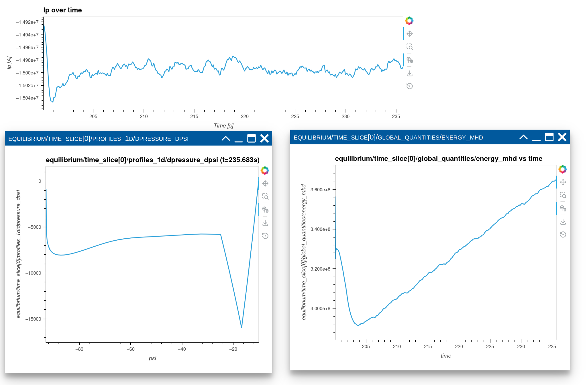
Run the MUSCLE pipeline, supplying the yMMSL file you made. Use the dropdown menu to visualize the following parameters:
equilibrium/time_slice[0]/profiles_1d[0]/dpressure_dpsiequilibrium/time_slice[0]/global_quantities/energy_mhd
Besides the plasma current curve, which was defined in the plotter class, you should also see the p' and the MHD energy curves in separate panels:
Exercise 3: Using the CLI
It is also possible to run the visualization actor from the command line instead, without setting up a MUSCLE3 workflow. Try running the simple_1d_plot example through the CLI.
Run the visualization with:
URI:
imas:hdf5?path=/home/ITER/blokhus/public/imasdb/ITER/4/666666/3/Plotting script:
imas_muscle3/visualization/examples/simple_1d_plot/simple_1d_plot.py
Hint
Use python -m imas_muscle3.visualization.cli --help to see available options.
Run the following command:
python -m imas_muscle3.visualization.cli \
    "imas:hdf5?path=/home/ITER/blokhus/public/imasdb/ITER/4/666666/3/" \
    imas_muscle3/visualization/examples/simple_1d_plot/simple_1d_plot.py
Exercise 4: Loading Machine Descriptions
In this exercise you will create a 2D plot that combines static machine description data with time-evolving equilibrium data. Specifically,
The plasma boundary outline (from the equilibrium IDS) as it changes over time.
The tokamak first wall and divertor (from the wall machine description IDS).
You will need to update your yMMSL from exercise 1a, with the following changes:
Add a new source actor which will send the
wallandpf_activemachine description IDSs to the visualization actor.- The new source actor should use the following URI:
imas:hdf5?path=/home/ITER/blokhus/public/imasdb/ITER/4/666666/3/
The visualization actor should receive the machine description IDSs on the S port, with the names
wall_md_inandpf_active_md_in.
You will need to implement the extract_equilibrium, _plot_boundary_outline, and _plot_wall methods, in the template below.
Implement the extract_equilibrium method which does the following:
Loads R and Z coordinates of the the boundary outline from the equilibrium IDS:
ids.time_slice[0].boundary.outline.r,ids.time_slice[0].boundary.outline.zStores both in an Xarray Dataset.
Either saves the first entry in
self.dataor concatenates it to an existing Dataset.
Implement the _plot_boundary_outline method which does the following:
Load the state data from the current
self.active_state.Extract the r and z arrays from the state data (use
state.sel(time=self.time)).Display r and z, using a HoloViews Curve.
Implement the _plot_wall method which does the following:
Load the wall machine description IDS using
self.active_state.md.get("wall").Loads the first wall and divertor from the wall IDS:
ids.description_2d[0].limiter.unit[i].outline.randids.description_2d[0].limiter.unit[i].outline.zfori = 0andi = 1.Display r and z, using a HoloViews Path.
import holoviews as hv
import numpy as np
import panel as pn
import xarray as xr

from imas_muscle3.visualization.base_plotter import BasePlotter
from imas_muscle3.visualization.base_state import BaseState


class State(BaseState):
    def extract(self, ids):
        if ids.metadata.name == "equilibrium":
            self.extract_equilibrium(ids)

    def extract_equilibrium(self, ids):
        # Implement this method!

class Plotter(BasePlotter):
    DEFAULT_OPTS = hv.opts.Overlay(
        xlim=(0, 13),
        ylim=(-10, 10),
        title="Wall and equilibrium boundary outline",
        xlabel="r [m]",
        ylabel="z [m]",
    )

    def get_dashboard(self):
        elements = [
            hv.DynamicMap(self._plot_boundary_outline),
            hv.DynamicMap(self._plot_wall),
        ]
        overlay = hv.Overlay(elements).collate().opts(self.DEFAULT_OPTS)
        return pn.pane.HoloViews(overlay, width=800, height=1000)

    @pn.depends("time")
    def _plot_boundary_outline(self):
        # Implement this method!

    def _plot_wall(self):
        # Implement this method!
Example yMMSL file:
ymmsl_version: v0.1
model:
  name: test_model
  components:
    source_component:
      implementation: source_component
      ports:
        o_i: [equilibrium_out]
    source_component_md:
      implementation: source_component
      ports:
        o_i: [wall_out, pf_active_out]
    visualization_component:
      implementation: visualization_component
      ports:
        s: [equilibrium_in, pf_active_md_in, wall_md_in]
  conduits:
    source_component.equilibrium_out: visualization_component.equilibrium_in
    source_component_md.wall_out: visualization_component.wall_md_in
    source_component_md.pf_active_out: visualization_component.pf_active_md_in
settings:
  source_component.source_uri: imas:hdf5?path=/home/ITER/blokhus/public/imasdb/ITER/4/666666/3/
  source_component_md.source_uri: imas:hdf5?path=/home/ITER/blokhus/public/imasdb/ITER/4/666666/3/
  visualization_component.plot_file_path: /home/ITER/blokhus/projects/IMAS-MUSCLE3/imas_muscle3/visualization/examples/machine_description/machine_description.py
  visualization_component.keep_alive: true
implementations:
  visualization_component:
    executable: python
    args: -u -m imas_muscle3.actors.visualization_component
  source_component:
    executable: python
    args: -u -m imas_muscle3.actors.source_component
resources:
  source_component:
    threads: 1
  source_component_md:
    threads: 1
  visualization_component:
    threads: 1
Example plotting script:
"""
Example that plots the following:
- First wall and divertor from machine description IDS.
- Boundary outline from an equilibrium IDS
"""

import holoviews as hv
import numpy as np
import panel as pn
import xarray as xr

from imas_muscle3.visualization.base_plotter import BasePlotter
from imas_muscle3.visualization.base_state import BaseState


class State(BaseState):
    def extract(self, ids):
        if ids.metadata.name == "equilibrium":
            self.extract_equilibrium(ids)

    def extract_equilibrium(self, ids):
        ts = ids.time_slice[0]
        outline = ts.boundary.outline

        boundary_data = xr.Dataset(
            {
                "r": (("time", "point"), [outline.r]),
                "z": (("time", "point"), [outline.z]),
            },
            coords={
                "time": [ids.time[0]],
                "point": np.arange(len(outline.r)),
            },
        )

        current_data = self.data.get("equilibrium")
        if current_data is None:
            self.data["equilibrium"] = boundary_data
        else:
            self.data["equilibrium"] = xr.concat(
                [current_data, boundary_data], dim="time", join="outer"
            )


class Plotter(BasePlotter):
    DEFAULT_OPTS = hv.opts.Overlay(
        xlim=(0, 13),
        ylim=(-10, 10),
        title="Wall and equilibrium boundary outline",
        xlabel="r [m]",
        ylabel="z [m]",
    )

    def get_dashboard(self):
        elements = [
            hv.DynamicMap(self._plot_boundary_outline),
            hv.DynamicMap(self._plot_wall),
        ]
        overlay = hv.Overlay(elements).collate().opts(self.DEFAULT_OPTS)
        return pn.pane.HoloViews(overlay, width=800, height=1000)

    @pn.depends("time")
    def _plot_boundary_outline(self):
        state = self.active_state.data.get("equilibrium")

        if state is not None and "r" in state and "z" in state:
            selected_data = state.sel(time=self.time)
            r = selected_data.r.values
            z = selected_data.z.values
        else:
            r, z = [], [], "Waiting for data..."

        return hv.Curve((r, z)).opts(self.DEFAULT_OPTS)

    def _plot_wall(self):
        """Generates path for limiter and divertor."""
        paths = []
        wall = self.active_state.md.get("wall")
        if wall is not None:
            for unit in wall.description_2d[0].limiter.unit:
                name = str(unit.name)
                r_vals = unit.outline.r
                z_vals = unit.outline.z
                paths.append((r_vals, z_vals, name))
        return hv.Path(paths, vdims=["name"]).opts(
            color="black",
            line_width=2,
            hover_tooltips=[("", "@name")],
        )